
aridagri analyses the field experiments that agronomists and plant breeders run every season: CRD, RCBD, factorials, the whole split-plot family, strip plots, combined analysis over years and locations, augmented and alpha lattice trials, repeated measurements, and stability analysis. Each analysis gives the correct error term for every source, SEm, SEd, CD and CV, and letter groupings, in the form journals and theses ask for.
Website: https://lalitrolaniya.github.io/aridagri/
Installation
install.packages("aridagri")

# development version
# install.packages("remotes")
remotes::install_github("lalitrolaniya/aridagri")
A table for your paper in one call
library(aridagri)

tab <- anova_traits(mothbean_rbd,
                    traits = c("plant_height", "pods_per_plant",
                               "seed_yield", "harvest_index"),
                    design = "rbd", treatment = "treatment",
                    block = "block", posthoc = "duncan")
export_results(tab, "Table_2.xlsx")
treatment plant_height pods_per_plant seed_yield harvest_index
T1 Control 30.25 c 19.05 e 516.25 d 29.77
T2 RDF 33.33 ab 24.70 cd 604.75 c 30.30
...
T5 RDF+Rhizobium+PSB 35.00 a 29.10 a 705.00 a 32.33
SEm ± 0.63 0.75 15.60 0.77
CD (p = 0.05) 1.86 2.21 45.88 NS
CV (%) 3.77 5.93 4.97 4.91What it covers
Examples and figures
Most analyses have a plot() method, and there are dedicated functions for interaction, stability and response plots. Every figure is a ggplot2 object, so you can change labels or themes with + and save it with ggsave(). The example datasets are simulated.
Treatment means with letter groups
res <- anova_rbd(mothbean_rbd, "seed_yield", "treatment", "block",
                 posthoc = "duncan")
plot(res, ylab = "Seed yield (kg/ha)",
     title = "Moth bean seed yield (RCBD, DMRT)")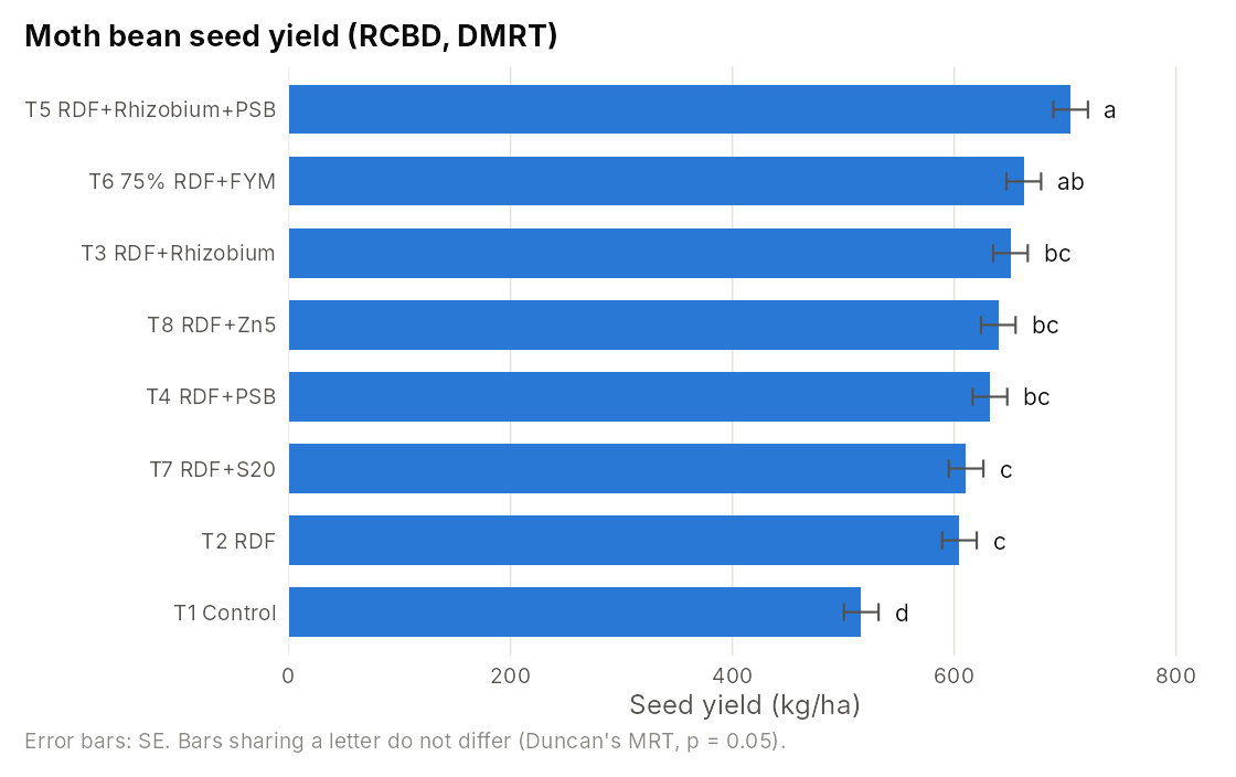
Split plot: Error(a), Error(b) and the four CDs
sp <- anova_spd(clusterbean_spd, "seed_yield", main_plot = "irrigation",
                sub_plot = "nitrogen", replication = "rep")
plot_interaction(sp, ylab = "Seed yield (kg/ha)",
                 title = "Cluster bean: irrigation x nitrogen")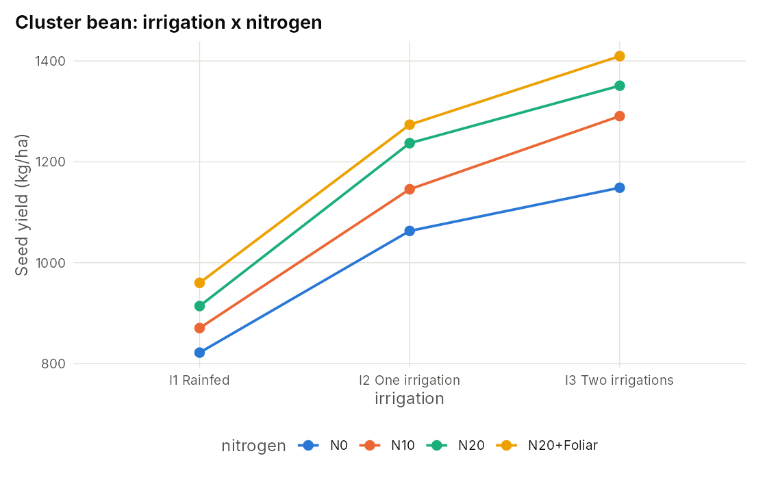
Stability over six environments
st <- stability_analysis(pearlmillet_met, "genotype", "environment",
                         "rep", "grain_yield")
plot_stability(st, "eberhart",
               title = "Pearl millet: mean yield vs regression slope")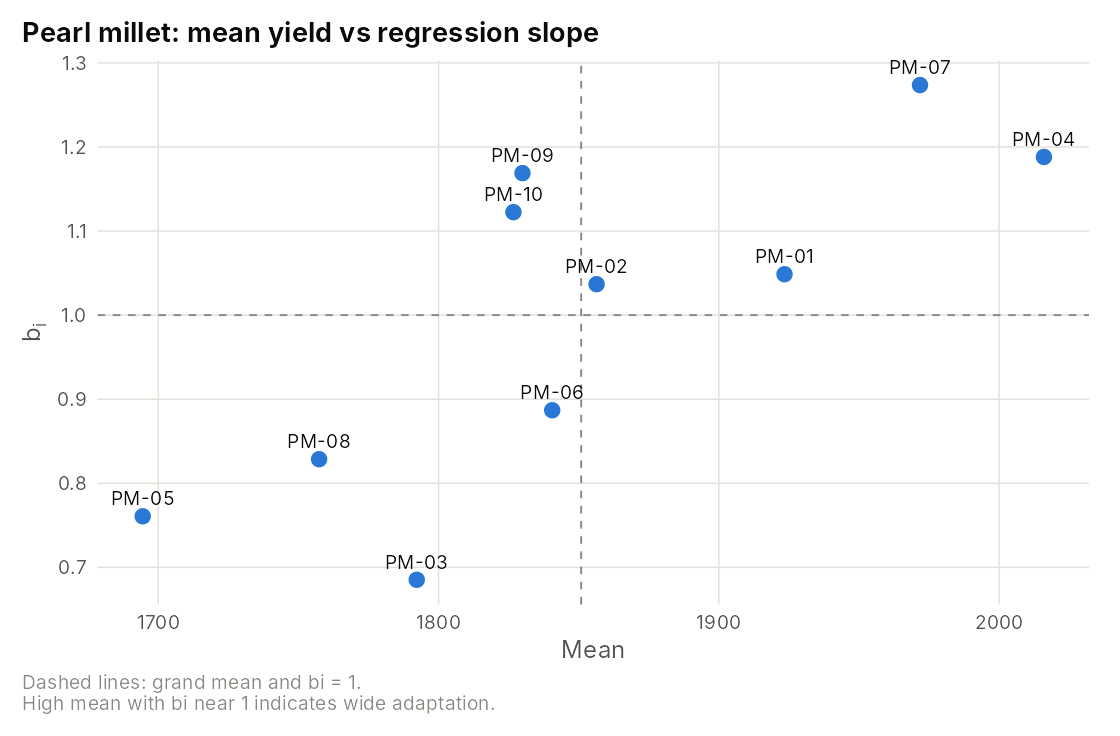
AMMI and GGE biplots come from the same data:
plot_stability(st, "ammi2")
gge <- gge_biplot(pearlmillet_met, "genotype", "environment", "grain_yield")
plot(gge, type = "which_won_where")
Germplasm in an augmented design
au <- anova_augmented(chickpea_augmented, "seed_yield", "entry", "block",
                      check_names = c("C1", "C2", "C3", "C4"))
plot(au, top = 15, ylab = "Adjusted seed yield (kg/ha)",
     title = "Chickpea germplasm: top 15 accessions and checks")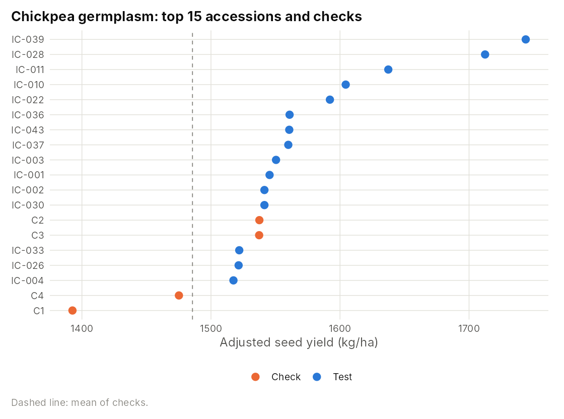
Repeated measurements on the same plots
rm <- anova_repeated(mungbean_repeated, "spad", "treatment", "das",
                     block = "block")
plot(rm, ylab = "SPAD reading", title = "Mung bean chlorophyll over time") +
  ggplot2::labs(x = "Days after sowing")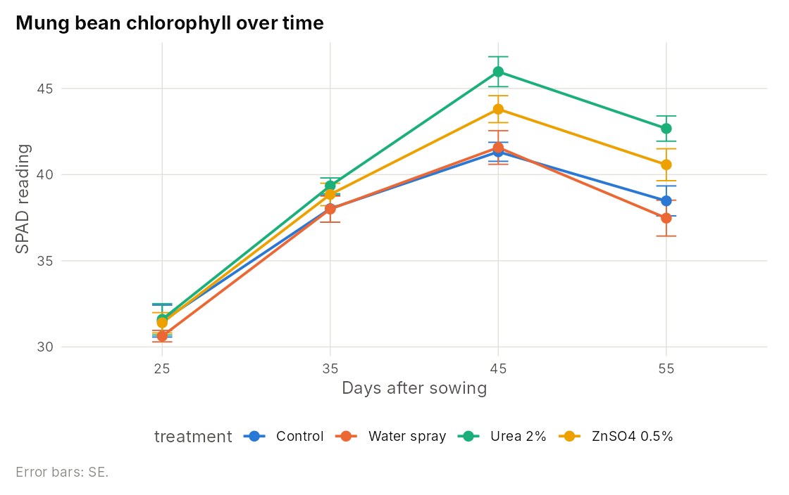
Nutrient response and economic optimum dose
dose  <- c(0, 20, 40, 60, 80, 100)
yield <- c(1100, 1350, 1520, 1610, 1650, 1660)
nr <- nutrient_response(dose, yield, model = "all",
                        price_output = 25, price_nutrient = 40)
plot_response(nr, dose, yield, title = "Nitrogen response: four models")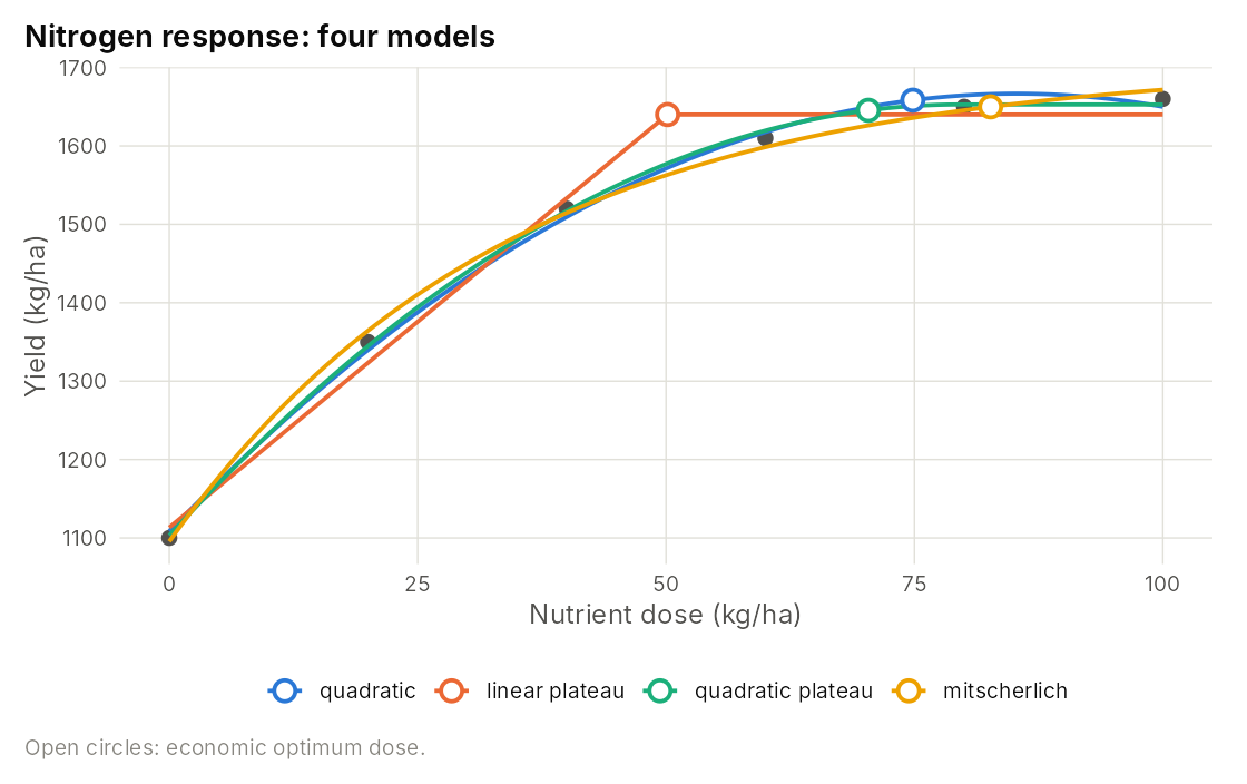
Letters from a published table
compare_means(c(T1 = 1180, T2 = 1265, T3 = 1342, T4 = 1410),
              mse = 3600, df_error = 12, reps = 4, method = "duncan")
What changed in 2.1.0
Version 2.1.0 corrects several calculations (relative efficiency in RCBD, the pooled RCBD error terms and silent mode, the strip-plot F-tests, the split-plot table returned to the user, Shukla’s variance, the AMMI stability value, Eberhart-Russell S2di, the variance test in check_assumptions(), and the utilization efficiency in nue_calculate()). If you used these functions in 2.0.x, please rerun the analyses. See NEWS for details.
All letter groupings are now computed in the package and agree with ‘agricolae’ on balanced data; unequal replication and missing plots are handled exactly. Results are tested against ‘agricolae’, ‘emmeans’, aov() error strata and base R’s sphericity tests (607 test expectations).
Citation
citation("aridagri")Rolaniya, L.K., Jat, R.L., Punia, M., Choudhary, R.R. and Poonia, H. (2026). aridagri: An R package for comprehensive statistical analysis of agricultural field experiments. Software Impacts, 29, 100851. https://doi.org/10.1016/j.simpa.2026.100851
Authors
| Author | Affiliation |
|---|---|
| Lalit Kumar Rolaniya (maintainer) | Scientist (Agronomy), ICAR-Indian Institute of Pulses Research, Regional Centre, Bikaner |
| Ram Lal Jat | Senior Scientist (Agronomy), ICAR-Indian Institute of Pulses Research, Regional Centre, Bikaner |
| Monika Punia (deceased) | Scientist (Genetics and Plant Breeding), ICAR-Indian Institute of Pulses Research, Regional Centre, Bikaner |
| Raja Ram Choudhary | Scientist (Agronomy), ICAR-Indian Institute of Groundnut Research, Regional Research Station, Bikaner |
| Hemant Poonia (deceased) | Assistant Professor, Department of Mathematics and Statistics, CCS Haryana Agricultural University, Hisar |
Version 2.1.0 is dedicated to the memory of our co-authors Dr. Monika Punia and Dr. Hemant Poonia.