Principal Component Analysis

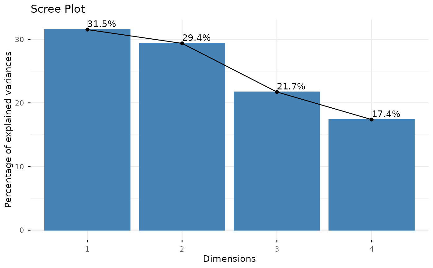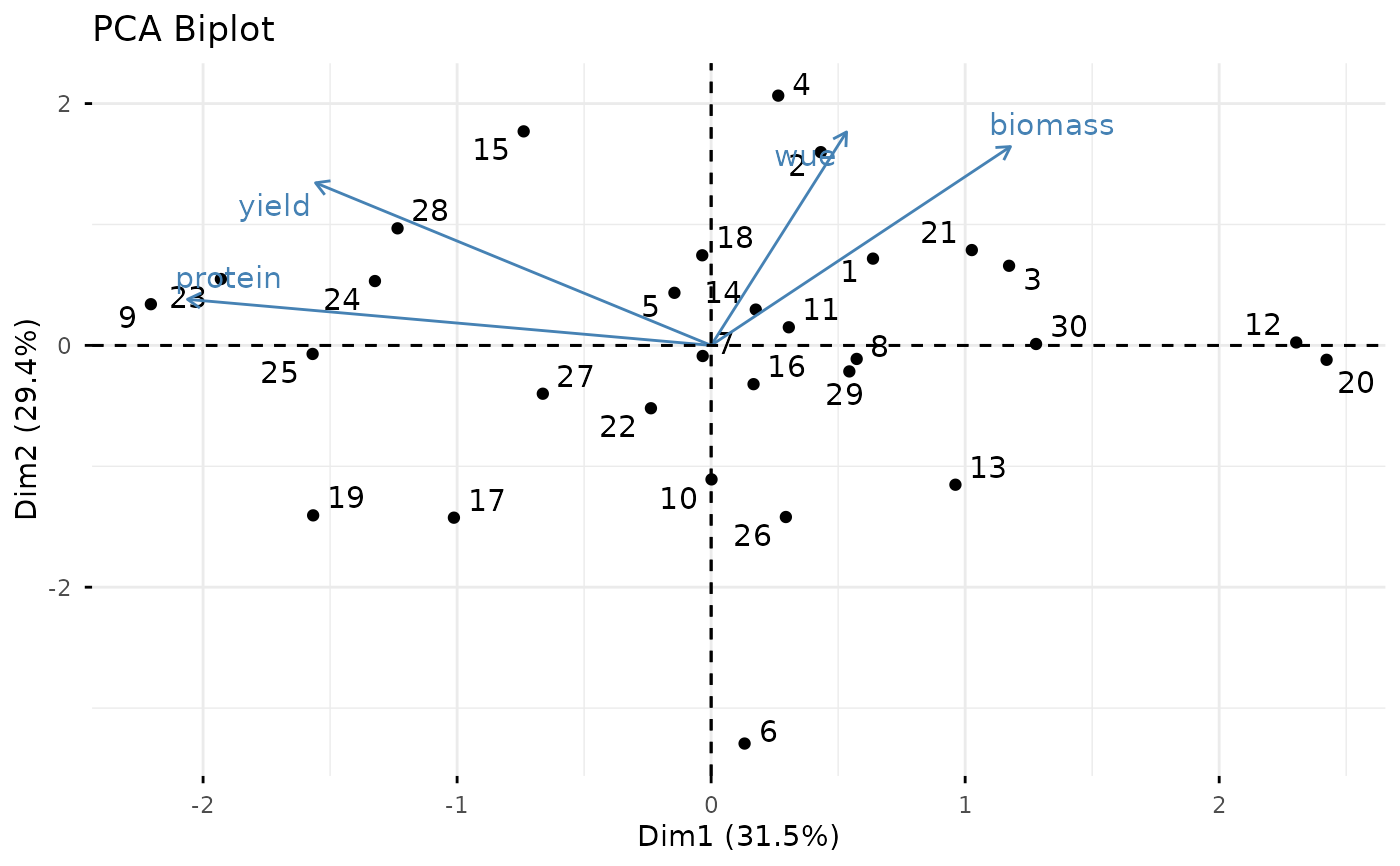
Performs PCA with visualization suitable for agricultural research data. Includes scree plot, biplot, and variable contributions.

Usage

pca_analysis(data, scale = TRUE, ncp = 5, plot = TRUE, verbose = TRUE)

Arguments

data

Data frame with numeric variables

scale

Logical, whether to scale variables (default TRUE)

ncp

Number of components to retain (default 5)

plot

Logical, whether to generate plots

verbose

Logical. If TRUE (default), prints formatted output to console.

Value

PCA results with eigenvalues, loadings, and scores

Author

Lalit Kumar Rolaniya, ICAR-IIPR, Bikaner

Examples

data <- data.frame(
  yield = rnorm(30, 1200, 200),
  wue = rnorm(30, 4.5, 0.5),
  protein = rnorm(30, 22, 2),
  biomass = rnorm(30, 3500, 500)
)
pca_analysis(data)
#> 
#> ==========================================================
#>           PRINCIPAL COMPONENT ANALYSIS
#> ==========================================================
#> Variables: 4 
#> Observations: 30 
#> Scaling: Yes 
#> 
#> --- Eigenvalues and Variance Explained ---
#> 
#>    PC Eigenvalue Variance_Percent Cumulative_Percent
#> 1 PC1      1.261            31.53              31.53
#> 2 PC2      1.175            29.36              60.89
#> 3 PC3      0.869            21.72              82.62
#> 4 PC4      0.695            17.38             100.00
#> 
#> --- Variable Loadings (First 3 PCs) ---
#> 
#>            PC1   PC2    PC3    PC4
#> yield   -0.539 0.482  0.408 -0.558
#> wue      0.184 0.633 -0.733 -0.166
#> protein -0.713 0.137 -0.210  0.654
#> biomass  0.408 0.590  0.502  0.483
#> 
#> --- Recommendation ---
#> Components retained by the Kaiser criterion: 2 
#> Variance explained by 2 components: 60.9 %