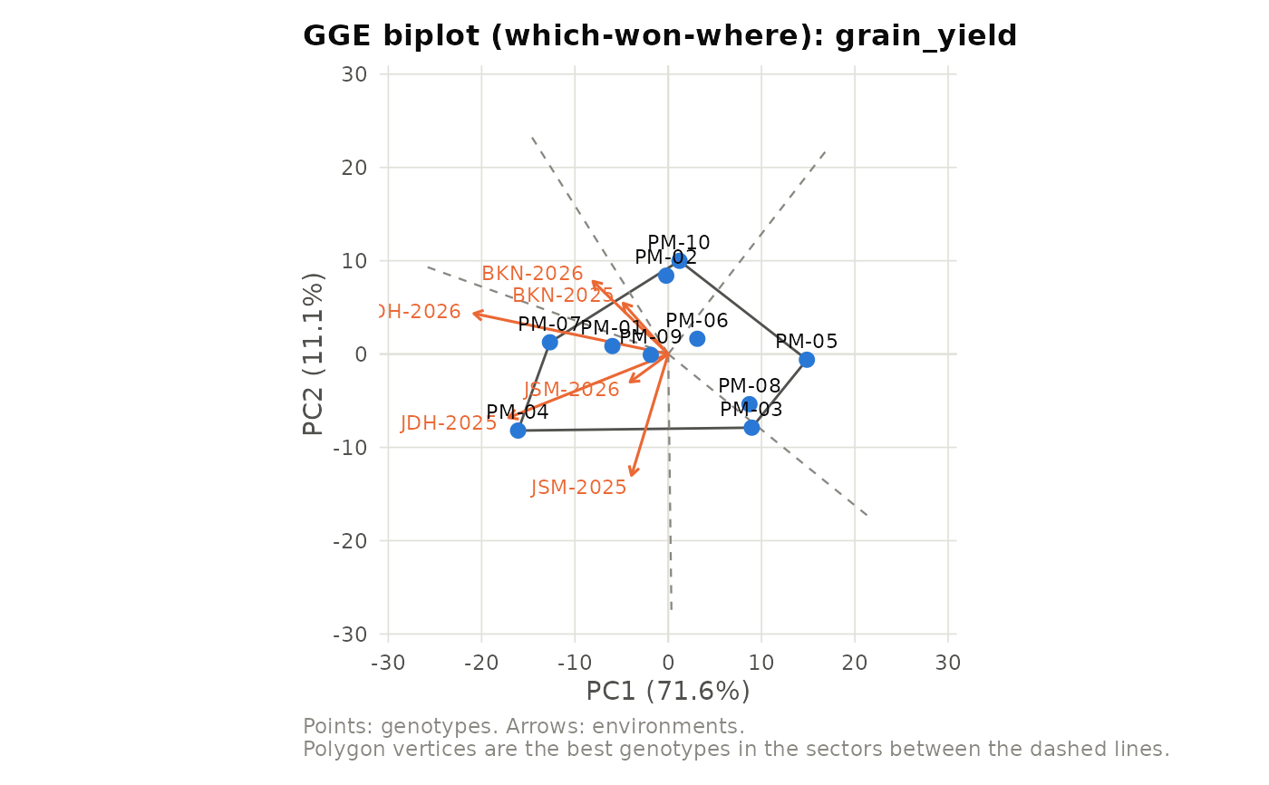
Genotype plus genotype-by-environment (GGE) biplot analysis of a multi-environment trial (Yan et al., 2000). Gives the genotype and environment scores on the first two principal components, the winning genotype in each environment and the resulting mega-environments (which-won-where), and the average-environment coordination (AEC) ranking of genotypes for mean performance and stability.
Arguments
- data
Data frame with genotype, environment and trait columns (plot data or genotype x environment means).
- genotype
Name of the genotype column.
- environment
Name of the environment column.
- trait
Name of the trait column.
- scaling
"none"(default) or"sd"(each environment divided by its standard deviation, giving environments equal weight).- svp
Singular value partitioning:
"symmetric"(default, suited to which-won-where),"genotype"(genotype-focused, suited to comparing genotypes and the mean vs stability view) or"environment"(environment-focused).- verbose
Logical. If TRUE (default), prints a summary.
Value
An object of class aridagri_gge with
genotype_scores, environment_scores,
variance_percent, which_won_where (environment and
winner), mega_environments, aec (genotype AEC abscissa,
ordinate and ranks) and the settings used. Plot it with
plot().
Details
The genotype x environment table of means is centred on the environment means (and optionally scaled) and decomposed by singular value decomposition. With singular values \(d_k\), genotype scores are \(u_{ik} d_k^f\) and environment scores \(v_{jk} d_k^{1-f}\), with \(f = 0.5, 1, 0\) for symmetric, genotype- and environment-focused partitioning. The winner in an environment is the genotype with the highest value predicted by the two-component biplot; environments with the same winner form a mega-environment. On the AEC view the abscissa (projection on the average-environment axis) ranks mean performance and the ordinate (distance from that axis) measures instability.
References
Yan, W., Hunt, L.A., Sheng, Q. and Szlavnics, Z. (2000). Cultivar evaluation and mega-environment investigation based on the GGE biplot. Crop Science, 40(3), 597-605. doi:10.2135/cropsci2000.403597x
Yan, W. and Kang, M.S. (2003). GGE Biplot Analysis: A Graphical Tool for Breeders, Geneticists, and Agronomists. CRC Press, Boca Raton.
Examples
data(pearlmillet_met)
gg <- gge_biplot(pearlmillet_met, "genotype", "environment", "grain_yield")
#>
#> ======================================================================
#>  GGE BIPLOT ANALYSIS
#> ======================================================================
#>  Trait                       : grain_yield
#>  Genotypes                   : 10
#>  Environments                : 6
#>  Scaling                     : none
#>  Singular value partitioning : symmetric
#>  PC1 + PC2                   : 82.7% of G + GE
#>
#>  Which won where
#>  Environment Winner
#>     BKN-2025  PM-07
#>     BKN-2026  PM-07
#>     JDH-2025  PM-04
#>     JDH-2026  PM-04
#>     JSM-2025  PM-04
#>     JSM-2026  PM-04
#>
#>  Mega-environments (environments sharing a winner)
#>   PM-04: JDH-2025, JDH-2026, JSM-2025, JSM-2026
#>   PM-07: BKN-2025, BKN-2026
#>
#>  Mean vs stability (average-environment coordination)
#>  Genotype     Mean AEC_abscissa AEC_ordinate Mean_rank Stability_rank
#>     PM-04 2016.000       16.756        6.751         1              7
#>     PM-07 1971.778       12.518        2.373         2              5
#>     PM-01 1923.444        5.888        1.382         3              3
#>     PM-09 1829.944        1.871        0.080         4              1
#>     PM-02 1856.389       -0.525        8.389         5              8
#>     PM-10 1826.722       -2.084        9.846         6             10
#>     PM-06 1840.556       -3.250        1.356         7              2
#>     PM-08 1757.389       -8.199        6.115         8              6
#>     PM-03 1792.222       -8.225        8.648         9              9
#>     PM-05 1694.444      -14.749        1.913        10              4
gg$which_won_where
#>   Environment Winner
#> 1    BKN-2025  PM-07
#> 2    BKN-2026  PM-07
#> 3    JDH-2025  PM-04
#> 4    JDH-2026  PM-04
#> 5    JSM-2025  PM-04
#> 6    JSM-2026  PM-04
if (requireNamespace("ggplot2", quietly = TRUE)) {
  plot(gg, type = "which_won_where")
}