
aridagri analyses the field experiments that agronomists and breeders
run every season. Every function takes a data frame and column names,
prints a report, and returns an object you can reuse. Set
verbose = FALSE to keep only the object.
The examples use six simulated datasets that ship with the package
(mothbean_rbd, clusterbean_spd,
pearlmillet_met, chickpea_augmented,
cowpea_alpha, mungbean_repeated). They mimic
arid-zone trials but are not real experimental results.
1. One trait in a randomized block design
res <- anova_rbd(mothbean_rbd, response = "seed_yield",
                 treatment = "treatment", block = "block",
                 posthoc = "duncan")
#>
#> ======================================================================
#>  RANDOMIZED COMPLETE BLOCK DESIGN (RCBD)
#> ======================================================================
#>  Response     : seed_yield
#>  Treatment    : treatment
#>  Treatments   : 8
#>  Blocks       : 4
#>  Observations : 32
#>
#>  Analysis of variance
#>     Source Df    Sum Sq  Mean Sq F value Pr(>F)
#>  Block      3  19781.59  6593.86   6.773 0.0023  **
#>  Treatment  7  84544.22 12077.75  12.405 0.0000 ***
#>  Error     21  20445.66   973.60
#>  Total     31 124771.47
#>  Signif. codes: *** p < 0.001, ** p < 0.01, * p < 0.05, NS not significant
#>
#>  Grand mean = 627.781   CV (%) = 4.970   SEm = 15.601   SEd = 22.064   CD (5%) = 45.884
#>  Relative efficiency of RCBD over CRD = 155.9%
#>
#>  Treatment means (Duncan's MRT, alpha = 0.05)
#>             Treatment   Mean     SD N     SE Group
#>  T5 RDF+Rhizobium+PSB 705.00 25.781 4 15.601     a
#>        T6 75% RDF+FYM 662.75 67.609 4 15.601    ab
#>      T3 RDF+Rhizobium 650.75 34.248 4 15.601    bc
#>            T8 RDF+Zn5 639.75 53.238 4 15.601    bc
#>            T4 RDF+PSB 632.25 26.887 4 15.601    bc
#>            T7 RDF+S20 610.75 26.247 4 15.601     c
#>                T2 RDF 604.75 49.815 4 15.601     c
#>            T1 Control 516.25 16.520 4 15.601     d
#>  Means sharing a letter do not differ significantly.
The report gives the ANOVA, SEm, SEd, CD at your alpha,
CV, the relative efficiency of blocking, and treatment means with
letters. Missing plots are handled by least squares: treatments are
tested after blocks and every pair of means is compared with its own
standard error.
plot(res, ylab = "Seed yield (kg/ha)")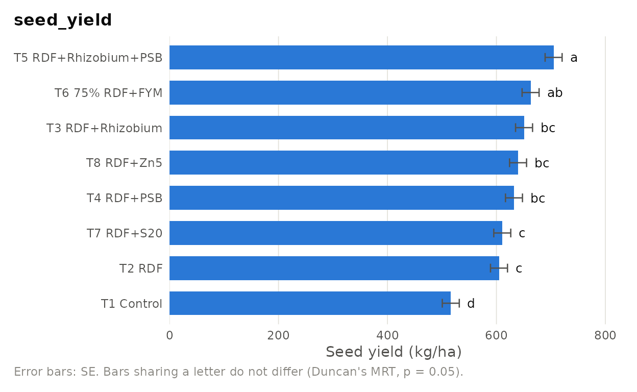
2. The table for your paper: many traits at once
tab <- anova_traits(mothbean_rbd,
                    traits = c("plant_height", "pods_per_plant",
                               "test_weight", "seed_yield", "harvest_index"),
                    design = "rbd", treatment = "treatment", block = "block",
                    posthoc = "duncan")
#>
#> ======================================================================
#>  TREATMENT MEANS FOR 5 TRAIT(S) (RBD)
#> ======================================================================
#>  treatment            plant_height pods_per_plant test_weight seed_yield
#>  T1 Control           30.25 c      19.05 e        28.27 c     516.25 d
#>  T2 RDF               33.33 ab     24.70 cd       29.23 b     604.75 c
#>  T3 RDF+Rhizobium     33.28 ab     25.10 cd       29.89 ab    650.75 bc
#>  T4 RDF+PSB           33.93 ab     26.42 bc       29.65 ab    632.25 bc
#>  T5 RDF+Rhizobium+PSB 35.00 a      29.10 a        30.25 a     705.00 a
#>  T6 75% RDF+FYM       35.17 a      27.80 ab       29.90 ab    662.75 ab
#>  T7 RDF+S20           34.48 ab     26.75 bc       29.96 ab    610.75 c
#>  T8 RDF+Zn5           32.90 b      23.75 d        29.48 ab    639.75 bc
#>  SEm ±                0.63         0.75           0.25        15.60
#>  CD (p = 0.05)        1.86         2.21           0.74        45.88
#>  CV (%)               3.77         5.93           1.70        4.97
#>  harvest_index
#>  29.77
#>  30.30
#>  32.00
#>  30.77
#>  32.33
#>  32.28
#>  30.83
#>  32.07
#>  0.77
#>  NS
#>  4.91
#>
#>  Means followed by the same letter do not differ significantly (Duncan's MRT, p = 0.05).
#>  NS: not significant. Full results for each trait are in $results.
Letters are dropped and CD is shown as NS when the F-test is not
significant. export_results(tab, "table.xlsx") writes the
table and the underlying statistics to Excel.
3. Split-plot designs with all four CDs
sp <- anova_spd(clusterbean_spd, response = "seed_yield",
                main_plot = "irrigation", sub_plot = "nitrogen",
                replication = "rep")
#>
#> ======================================================================
#>  SPLIT-PLOT TYPE DESIGN
#> ======================================================================
#>  Response     : seed_yield
#>  Design       : Split Plot Design
#>  Replications : 3
#>  Factors      : irrigation (3), nitrogen (4)
#>
#>  Analysis of variance
#>               Source Df     Sum Sq   Mean Sq F value Pr(>F)
#>  rep                  2    3154.39   1577.19   0.493 0.6437  NS
#>  irrigation           2 1057793.56 528896.78 165.238 0.0001 ***
#>  Error(a)             4   12803.28   3200.82
#>  nitrogen             3  209483.56  69827.85  89.389 0.0000 ***
#>  irrigation:nitrogen  6   15606.44   2601.07   3.330 0.0219   *
#>  Error(b)            18   14061.00    781.17
#>  Total               35 1312902.22
#>  Signif. codes: *** p < 0.001, ** p < 0.01, * p < 0.05, NS not significant
#>
#>  Grand mean = 1123.778
#>   Error(a) [main]: df = 4, MS = 3200.8194, CV = 5.03%
#>   Error(b) [sub]: df = 18, MS = 781.1667, CV = 2.49%
#>
#>  SEm, SEd and CD (alpha = 0.05)
#>  Comparison                                          SEm    SEd    CD     Error
#>  irrigation means                                    16.332 23.097 64.127 Ea
#>  nitrogen means                                       9.316 13.175 27.681 Eb
#>  irrigation levels at the same or different nitrogen 21.495 30.398 75.719 Ea+Eb
#>  nitrogen levels at the same irrigation              16.137 22.821 47.944 Eb
#>  CD for comparisons mixing error terms uses the weighted t of Cochran and Cox.
#>
#>  Means of irrigation (Fisher's LSD)
#>               Level    Mean Group
#>          I1 Rainfed  891.50     c
#>   I2 One irrigation 1179.83     b
#>  I3 Two irrigations 1300.00     a
#>
#>  Means of nitrogen (Fisher's LSD)
#>       Level    Mean Group
#>          N0 1011.11     d
#>         N10 1102.22     c
#>         N20 1167.33     b
#>  N20+Foliar 1214.44     a
#>
#>  Interaction means: irrigation x nitrogen
#>                         N0     N10  N20 N20+Foliar
#> I1 Rainfed          821.67  870.33  914     960.00
#> I2 One irrigation  1063.00 1145.67 1237    1273.67
#> I3 Two irrigations 1148.67 1290.67 1351    1409.67
The SE table covers the four comparisons of Gomez and Gomez (1984), including main-plot means at the same sub-plot level, which mixes Error(a) and Error(b) and uses the weighted t value. The same engine runs the split-plot designs with factorial main or sub-plots, the split-split-plot and the combined analyses over years.
plot_interaction(sp, ylab = "Seed yield (kg/ha)")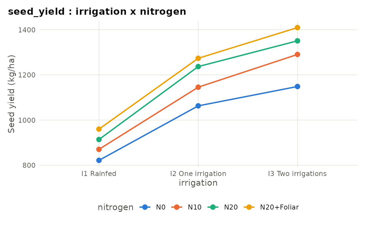
4. Several environments: pooled analysis, stability and GGE biplot
pool <- anova_rbd_pooled(pearlmillet_met, response = "grain_yield",
                         treatment = "genotype", environment = "environment",
                         block = "rep", verbose = FALSE)
pool$bartlett_test[c("chi_sq", "p_value")]
#> $chi_sq
#> [1] 5.375261
#>
#> $p_value
#> [1] 0.3718179
pool$pooled_anova
#>                       Df     Sum Sq    Mean Sq    F value       Pr(>F)
#> environment            5 21126520.4 4225304.08 198.051226 4.253250e-11
#> rep(environment)      12   256012.8   21334.40   2.042170 2.705284e-02
#> genotype               9  1529257.1  169917.46  16.264830 1.408097e-16
#> environment:genotype  45  1479461.6   32876.92   3.147043 6.349451e-07
#> Residuals            108  1128267.9   10446.92         NA           NA
st <- stability_analysis(pearlmillet_met, genotype = "genotype",
                         environment = "environment", replication = "rep",
                         trait = "grain_yield", verbose = FALSE)
st$eberhart[, c("Genotype", "Mean", "bi", "p_bi", "S2di", "p_S2di")]
#>    Genotype     Mean        bi       p_bi        S2di      p_S2di
#> 1     PM-04 2016.000 1.1880996 0.25330783 10534.45696 0.004410734
#> 2     PM-07 1971.778 1.2736153 0.01716838   -60.90468 0.420305801
#> 3     PM-01 1923.444 1.0486126 0.44159847 -1196.47687 0.623619365
#> 4     PM-02 1856.389 1.0367699 0.78794498  8029.50826 0.013473999
#> 5     PM-06 1840.556 0.8868424 0.13950632  -820.54307 0.550702395
#> 6     PM-09 1829.944 1.1689030 0.06031524  -500.74246 0.492837445
#> 7     PM-10 1826.722 1.1224747 0.31843257  4665.75834 0.059666052
#> 8     PM-03 1792.222 0.6852660 0.03414925  3498.86293 0.098943369
#> 9     PM-08 1757.389 0.8286463 0.14774463  2962.45905 0.124425636
#> 10    PM-05 1694.444 0.7607702 0.01254563 -1312.73413 0.647062473
st$ammi$anova
#>                         Df      Sum Sq    Mean Sq    F value       Pr(>F)
#> Environment              5 21126520.38 4225304.08 198.051226 4.253250e-11
#> Rep(Environment)        12   256012.80   21334.40   2.042170 2.705284e-02
#> Genotype                 9  1529257.11  169917.46  16.264830 1.408097e-16
#> Genotype x Environment  45  1479461.62   32876.92   3.147043 6.349451e-07
#>   IPCA1                 13   823910.41   63377.72   6.066639 2.245488e-08
#>   IPCA2                 11   329345.65   29940.51   2.865964 2.457518e-03
#>   IPCA3                  9   155354.79   17261.64   1.652318 1.095895e-01
#>   IPCA4                  7   113089.95   16155.71   1.546456 1.594051e-01
#>   IPCA5                  5    57760.82   11552.16   1.105796 3.616571e-01
#> Pooled error           108  1128267.87   10446.92         NA           NA
plot_stability(st, "eberhart")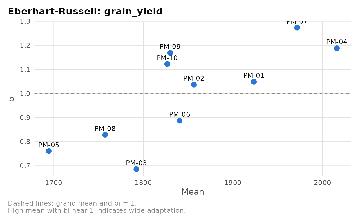
plot_stability(st, "ammi2")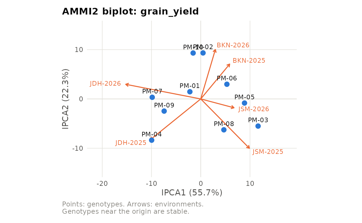
gg <- gge_biplot(pearlmillet_met, "genotype", "environment", "grain_yield",
                 verbose = FALSE)
gg$which_won_where
#>   Environment Winner
#> 1    BKN-2025  PM-07
#> 2    BKN-2026  PM-07
#> 3    JDH-2025  PM-04
#> 4    JDH-2026  PM-04
#> 5    JSM-2025  PM-04
#> 6    JSM-2026  PM-04
plot(gg, type = "which_won_where")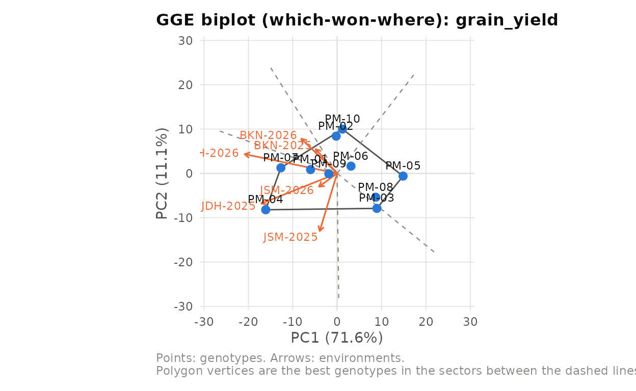
5. Germplasm evaluation: augmented and alpha lattice designs
au <- anova_augmented(chickpea_augmented, response = "seed_yield",
                      genotype = "entry", block = "block",
                      check_names = c("C1", "C2", "C3", "C4"),
                      verbose = FALSE)
head(au$test_vs_checks[, c("Entry", "Adjusted_mean", "Pct_over_best_check",
                           "Sig_vs_best")])
#>    Entry Adjusted_mean Pct_over_best_check Sig_vs_best
#> 1 IC-039      1743.917           13.425474      higher
#> 2 IC-028      1712.417           11.376694      higher
#> 3 IC-011      1637.417            6.498645          ns
#> 4 IC-010      1604.417            4.352304          ns
#> 5 IC-022      1592.167            3.555556          ns
#> 6 IC-036      1560.917            1.523035          ns
au$genetic_parameters
#>                        Parameter        Value
#> 1                  Mean of tests  1416.958333
#> 2                    Range (min)  1151.916667
#> 3                    Range (max)  1743.916667
#> 4            Phenotypic variance 19058.687352
#> 5             Genotypic variance 15708.842908
#> 6                 Error variance  3349.844444
#> 7                        PCV (%)     9.742926
#> 8                        GCV (%)     8.845350
#> 9  Heritability (broad sense, %)    82.423530
#> 10               Genetic advance   234.745314
#> 11               GA as % of mean    16.566847
al <- anova_alpha_lattice(cowpea_alpha, response = "grain_yield",
                          genotype = "genotype", replication = "rep",
                          block = "block", verbose = FALSE)
al$efficiency
#> [1] 166.7754
head(al$genotype_means)
#>   Genotype     Mean Adjusted_mean       SE Group
#> 1    CP-03 1229.667      1210.688 42.57639     a
#> 2    CP-17 1216.667      1163.069 42.57639   abc
#> 3    CP-16 1179.667      1162.403 42.59500    ab
#> 4    CP-12 1098.667      1108.596 42.59500   bcd
#> 5    CP-14 1097.333      1103.796 42.57639  bcde
#> 6    CP-09 1063.000      1094.972 42.59500 bcdef
6. Repeated measurements on the same plots or animals
rm <- anova_repeated(mungbean_repeated, response = "spad",
                     treatment = "treatment", time = "das", block = "block",
                     verbose = FALSE)
rm$sphericity
#>   Mauchly_W   p_value GG_epsilon HF_epsilon lower_bound
#> 1 0.5413907 0.4518438  0.7683995          1   0.3333333
rm$corrected
#>          Source Df    F_value p_uncorrected         p_GG         p_HF
#> 1           das  3 417.333071  1.013322e-22 6.414395e-18 1.013322e-22
#> 2 treatment:das  9   4.698104  8.219324e-04 2.793023e-03 8.219324e-04
#>    recommended
#> 1 1.013322e-22
#> 2 8.219324e-04
rm$covariance_models
#>   Structure Parameters      AIC      BIC    logLik
#> 1        CS         21 238.6950 276.6349 -98.34750
#> 2       AR1         21 230.7225 268.6625 -94.36127
#> 3        UN         29 238.5023 290.8955 -90.25116
plot(rm, ylab = "SPAD reading")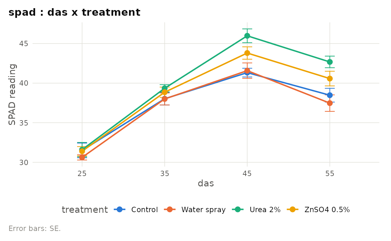
7. Agronomic indices
thermal_indices(tmax = c(31, 33, 35, 36, 38), tmin = c(16, 17, 19, 20, 22),
                base_temp = 10, sunshine_hours = rep(9.5, 5),
                day_length = day_length(28, 70:74), crop_yield = 1250)
#>
#> ======================================================================
#>  THERMAL INDICES
#> ======================================================================
#>  Days = 5   Base temperature = 10.0 C   Mean Tmax = 34.6 C   Mean Tmin = 18.8 C
#>
#>  Index                                Value   Unit
#>  Growing degree days (GDD)             83.500 degree C day
#>  Mean daily GDD                        16.700 degree C day per day
#>  Helio-thermal units (HTU)            793.250 degree C day hour
#>  Photo-thermal units (PTU)            981.619 degree C day hour
#>  Heat use efficiency (grain)           14.970 kg/ha per degree C day
#>  Helio-thermal use efficiency (grain)   1.576 kg/ha per degree C day hour

nue_calculate(yield_fertilized = c(1450, 1720, 1850), yield_control = 1200,
              nutrient_applied = c(20, 40, 60),
              nutrient_uptake_fert = c(48, 61, 68),
              nutrient_uptake_ctrl = 35)
#>
#> ======================================================================
#>  NUTRIENT USE EFFICIENCY
#> ======================================================================
#>  Yield_Fertilized Yield_Control Nutrient_Applied Yield_Response AE_kg_kg
#>              1450          1200               20            250    12.50
#>              1720          1200               40            520    13.00
#>              1850          1200               60            650    10.83
#>  PFP_kg_kg ARE_percent PE_kg_kg IE_kg_kg
#>      72.50          65    19.23    30.21
#>      43.00          65    20.00    28.20
#>      30.83          55    19.70    27.21
#>
#>  AE, PFP, PE, IE: kg grain per kg nutrient; ARE: percent of applied nutrient recovered

nr <- nutrient_response(dose = c(0, 20, 40, 60, 80, 100),
                        yield = c(1100, 1350, 1520, 1610, 1650, 1660),
                        model = "all", price_output = 60,
                        price_nutrient = 15)
#>
#> ======================================================================
#>  NUTRIENT RESPONSE: MODEL COMPARISON
#> ======================================================================
#>              Model    R2 Adj_R2   RMSE    AIC Dose_max Max_yield Dose_economic
#>          quadratic 0.997  0.995 10.511 36.229   85.256  1666.693        83.628
#>     linear_plateau 0.990  0.983 20.276 44.113   50.159  1640.000        50.159
#>  quadratic_plateau 0.999  0.999  5.750 28.990   79.580  1652.843        78.139
#>       mitscherlich 0.998  0.996  9.519 35.040       NA  1704.850       146.460
#>  Yield_economic
#>        1666.489
#>        1640.000
#>        1652.663
#>        1696.258
#>
#>  Best model by AIC: quadratic_plateau
plot_response(nr, c(0, 20, 40, 60, 80, 100),
              c(1100, 1350, 1520, 1610, 1650, 1660))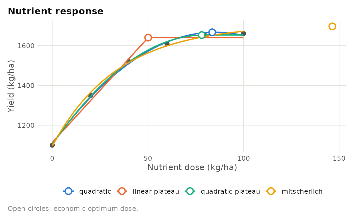
8. Letters from a published table
When you only have treatment means, the error mean square and its
degrees of freedom, compare_means() gives the letters:
compare_means(c(T1 = 1180, T2 = 1265, T3 = 1342, T4 = 1410, T5 = 1238),
              mse = 3600, df_error = 12, reps = 4, method = "duncan")
#>
#> Duncan's MRT (alpha = 0.05, error df = 12)
#> Critical ranges: p=2 92.439, p=3 96.757, p=4 99.374, p=5 101.105
#>  level mean SE group n
#>     T4 1410 30     a 4
#>     T3 1342 30    ab 4
#>     T2 1265 30    bc 4
#>     T5 1238 30     c 4
#>     T1 1180 30     c 4
#>
#> Means sharing a letter do not differ significantly.